A whistle-stop tour of ORBTrace Mini’s tracing capabilities

For this walk-through we’ll use the trivially simple, err…simple, app from orbmule. You can clone that repository and compile that (in the examples/simple directory). The default options will give you a binary and supporting elf file configured for debugging, so let’s do that first;

$ cd orbmule/examples/simple
$ make
Compiling src/itm_messages.c
Compiling src/main.c
Assembling system/startup_ARMCM4.S
text data bss dec hex filename
1512 1080 10072 12664 3178 ofiles/simple.elf

Your numbers might vary slightly depending on what version of the compiler you’re using and what chip you’re targeting, but the principles should hold. Now, let’s set up gdb to load this into our target automatically on startup. There are a number of gdbinit files for different probes in the gdbinit directory. We’re going to use the one for blackmagic;

$ cp gdbinit_files/gdbinit-bmp .gdbinit

Now, assuming you’ve got ORBTrace connected, it should just be a case of starting blackmagic, and the debugger. In the first window;

$ ./blackmagic
Listening on TCP: 2000

…and in the second;

$ arm-none-eabi-gdb -q
0xfffffffe in ?? ()
Available Targets:
No. Att Driver
1 STM32F40x M4
A program is being debugged already. Kill it? (y or n) [answered Y; input not from terminal]
0xfffffffe in ?? ()
Loading section .text, size 0x5e0 lma 0x8000000
Loading section .ARM.exidx, size 0x8 lma 0x80005e0
Loading section .data, size 0x438 lma 0x80005e8
Start address 0x80002a4, load size 2592
Transfer rate: 11 KB/sec, 518 bytes/write.
$1 = 1
(gdb)

You’re good. From this point you’ve got a full set of debugging goodness available to you, but we’ve covered that before so let’s move on. You will have noticed the TRACE led on ORBTrace goes red when the application is running…that’s because TRACE data are being created, but aren’t yet being consumed by the host. There are actually two streams of useful data being generated; One is the equivalent of the output you would get from SWO (Software messages, Program counter samples etc), and the second one is full TRACE. The orbuculum mux will capture those and publish them on consecutive TCP ports. Lets get it started;

$ orbuculum -t 1,2
Started Network interface for channel 1 on port 3443
Started Network interface for channel 2 on port 3444

(You can start this with the -v2 option if you prefer to see a little bit more of what is going on).

We are now ready to start consuming those rich data feeds to tell us more about what our CPU is doing.

Decoding software messages

First of all, let’s collect the software messages. This has already been covered in a previous article, but it’s worth the recap. The simple app is reciting the alphabet on channel 0, so in yet another window (you’ll learn to appreciate the benefits of screen or tmux quite quickly when you’re doing this stuff) lets collect and display those data;

$ orbcat -c 0,"%c"
VWXYABCDEFGHIJKLMNOPQRSTUVWXYABCDEFGHIJKLMNOPQRSTUVWXYABCDEFGHIJKLMNOPQRSTUVWXYABCDEFGHIJKLMNOPQRSTUVWXYABCDEFGHIJKLMNOPQRSTUVWXYABCDEFGHIJKLMNOPQRSTUVWXYABCDEFGHIJKLMNOPQRSTUVWXYABCDEFGHIJKLMNOPQRSTUVWXYABCDEFGHIJKLMNOPQRSTUVWXYABCDEFGHIJKLMNOPQRSTUVWXYABCDEFGHIJKLMNOPQRSTUVWXYABCDEFGHIJKLMNOPQRSTUVWXYABCDEFGHIJKLMNOPQRSTUVWXYABCDEFGHIJKLMNOPQRSTUVWXYABCDEFGHIJKLMNOP

You can choose the format you want, so you might prefer to see them as hex ASCII, for example;

$ orbcat -c 0,"%02x "
46 47 48 49 4a 4b 4c 4d 4e 4f 50 51 52 53 54 55 56 57 58 59 41 42 43 44 45 46 47 48 49 4a 4b 4c 4d 4e 4f 50 51 52 53 54 55 56 57 58 59 41 42 43 44 45 46 47 48 49 4a 4b 4c 4d 4e 4f 50 51 52 53 54 55 56 57 58 59 41 42 43 44 45 46 47 48 49 4a 4b 4c 4d 4e 4f 50 51 52 53 54 55 56 57 58 59 41 42 43 44 45 46 47 48 49 4a 4b 4c 4d 4e 4f 50 51 52 53 54 55 56 57 58 59 41 42 43 44 45 46 47 48 49 4a 4b 4c 4d 4e 4f 50 51 52 53 54 55 56 57 58 59 41 42 43 44 45 46 47 48 49 4a 4b 4c 4d 4e 4f 50 51 52 53 54 55 56 57 58 59 41 42 43 44 45 46 47 48 49 4a 4b 4c 4d 4e 4f 50 51 52 53 54 55 56 57 58 59 41 42

…or perhaps as ASCII, Hex and decimal representations (You can have up to 4 parallel decodes for an 8 bit value);

$ orbcat -c 0,"%c %02x %3d \n"
K 4b 75
L 4c 76
M 4d 77
N 4e 78
O 4f 79
P 50 80
Q 51 81
R 52 82

Of course, you can even do these things simultaneously, or pipe the output of orbcat to a graphing program or similar. There are 32 of these channels available, so you can create quite complex and feature-full output (and orbcat supports multiple -c options on one command line, so you can mix and match channels as you wish).

Decoding Hardware messages

Alongside the software messages, this target has also been configured to output program counter values in the gdbinit you copied over. With a knowledge of the application that is running on the target, we can use that to figure out what the application is doing over time, in a manner akin to the ‘top’ application on a PC. This simple application is so trivial that we’ll split it out by line number, but fiddle with the command line options to see the things that are possible;

$ orbtop -l -e orbmule/examples/simple/ofiles/simple.elf
24.48%     345 _sieve::39
23.20%     327 _sieve::41
19.23%     271 _sieve
7.87%      111 _sieve::32
7.73%      109 _sieve::30
5.89%       83 _sieve::45
4.82%       68 _sieve::47
4.32%       61 _sieve::42
1.41%       20 _sieve::38
0.85%       12 _sieve::36
0.14%        2 _sieve::44
--------------
99.94% 1409 of 1409 Samples
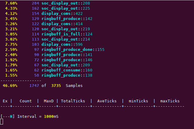
[-S-H] Interval = 1000mS

This can, of course, be running at the same time as the text messages are being printed out, and you can fiddle with chip configuration to get more or less samples, and program configuration to aggregate by line or function. You can also monitor what interrupts are being executed and how long they are taking to be processed. As an example of something slightly more complex, here’s a screenshot of orbtop monitoring the lcd_demo application that is also in the orbmule repository;

Program post-mortem

Finally, we’ll take a very quick look at the other stream of information that is being delivered by the probe. While the program is running a continuous report of program execution is generated. Orbmortem captures this into a ring buffer, so that when the program stops, we can tell exactly what instructions were executed up to that point. Typically this stop might be on a program counter value (e.g. hitting the hardfault handler) or because a specific variable has been modified. As a simple example, we’ll just stop on a CTRL-C to the debugger. In the gdb window type startETM to enable this data flow then, in another window, type;

$ orbmortem -e ~/Develop/orb/orbmule/examples/simple/ofiles/simple.elf

This will start the background capturing process which, admittedly, doesn’t look too impressive;

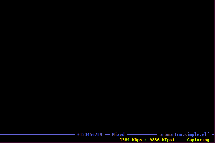
However, if you now hit CTRL-C in the debugger, things quickly get a lot more interesting;

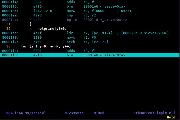
This window shows you the last instruction the chip executed before it stopped…if you look in the debugger it will show the address as being 0x080001e6 since that is the next instruction to be executed. From here you can scroll backwards and forwards through the post-mortem buffer (in this case through the last half million or so instructions), and search for particular events in Source, Assembly or Mixed (the default) views. You can also place markers and ‘dive into’ the source code itself using the left and right arrow keys. Finally, provided you set up the correct options on the command line, you can even open your favourite editor at a specific line in the execution view. For anyone who has ever ended up in ‘Hardfault Hell’ with no idea how they got there, this is gonna be a godsend!

Wrapping up

So, there you have it, a whistle-stop tour of the key capabilities of ORBTrace. It’s very much a work in progress. I’m sure it has bugs and I’m equally sure we’ve only just scratched the surface of what we can do with it.

Come join us.